About the Online Map

If your drawing contains geographic location information, and you are signed in to Autodesk 360, you can display a map from an online maps service in the current viewport.

The online map is a temporary graphic that is dynamically supplied by the online maps service. It displays behind all other drawing objects in the viewport and covers the extent of the GIS coordinate system assigned to the drawing file. Since the online map is a temporary graphic, you cannot plot the online map, and cannot be displayed if you are not signed in to Autodesk 360. Another drawback of the online map is that it usually covers a large area; much larger than the scope of a typical CAD project.

If you need to plot a map, or display the map when you are offline, you can "capture" the area you are interested in, to an object known as a map image. The map image embeds itself to the drawing area on top of the online map and is saved with the drawing. Unlike the online map, the map image is not a temporary graphic, and hence you can plot it. It is available even if you are not signed in to Autodesk 360.

Map Styles

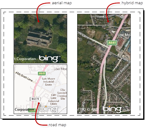
You can display the map as a satellite image (aerial style map) or as a vector image (road style map). You can also display the map as a hybrid of the aerial and road styles. If the drawing area is divided into multiple viewports, each viewport can have a different style of map.

Use of Map in Dialog Boxes

The online map also displays in the Geographic Location dialog box. It gives you the ability to pick a reference point to use as the geographic marker. If you want to limit the amount of data downloaded to your computer, you can choose not use live map data. When you do so, the system does not connect to the maps service and the maps behave as though you are not connected to the Internet.

Note: We recommend that you use a 64-bit system to work with the online map. Using the online map on a 32-bit system may cause the system to slow down.

Export Storm Sewers .stm Files From Autodesk Civil 3D

You can export one or more pipe networks into an .stm file. You must choose entire pipe networks. You cannot export individual parts, or a set of connected parts within a pipe network.

The .stm file can then be opened by the Hydraflow Storm Sewers extension for analysis and editing. After editing the file in Storm Sewers, you can import it back into Autodesk Civil 3D. Changes made to the file while in the Storm Sewers extension are recognized in Autodesk Civil 3D.

To export an .stm file from Autodesk Civil 3D

1. Click Output tabExport panelExport To Storm Sewers  Find.
2. On the Export to Storm Sewers dialog box, specify the pipe networks to be exported, and then click OK.
3. On the Export Storm Sewers to File dialog box, specify the location and the name for the .stm file, and then click Save.

To export an .stm file from Autodesk Civil 3D and open it in Storm Sewers for editing

1. Click Analyze tabDesign panel Edit In Storm Sewers  Find.
2. On the Export to Storm Sewers dialog box, specify the pipe networks to be exported, and then click OK.
3. On the Export Storm Sewers to File dialog box, specify the location and the name for the .stm file, and then click Save.

Hydraulics and Hydrology Features

Autodesk Civil 3D includes additional software applications that allow you to perform a variety of storm water management tasks, including storm sewer design, watershed analysis, detention pond modeling, and culvert, channel, and inlet analysis.

External applications can be used to add hydraulics and hydrology property information to Autodesk Civil 3D pipe networks. It is also possible to add hydraulics and hydrology property information directly to Autodesk Civil 3D pipe networks.

The applications are typically installed by default when you install Autodesk Civil 3D. If you chose not to install them when you first installed Autodesk Civil 3D, they can be installed later using Add or Remove Programs from the Control Panel.

The following table describes the hydraulics and hydrology extensions available with Autodesk Civil 3D.

Application	Description
Autodesk Storm and Sanitary Analysis	Autodesk® Storm and Sanitary Analysis is a comprehensive hydrology and hydraulic analysis application. It helps you plan and design urban drainage systems, storm sewers (including highway drainage systems), and sanitary sewers. Autodesk Storm and Sanitary Analysis integrates stormwater and wastewater analysis during planning and design, which helps you improve overall project productivity and increase your engineering capabilities.
Hydraflow Storm Sewers Extension	Enables you to perform storm sewer design and analysis on pipe network models. It is designed primarily for hydraulic and hydrologic analysis of simple and complex storm sewer networks with pavement drainage and inlet analysis. It can also be used as to determine the hydraulic grade line in an existing system, or for planning or designing new systems. Using Storm Sewers, you can add hydraulic information, such as hydraulic grade lines and energy grade lines, to Autodesk Civil 3D pipe network models.
Hydraflow Hydrographs Extension	Used for detention pond design and modeling of simple or complex watersheds using the SCS and/or Rational methods. This extension lets you perform a host of functions, including hydrograph combining, channel reach and pond routing, and hydrograph diverting.
Hydraflow Express Extension	Provides a collection of calculators for solving hydraulics and hydrology tasks on culverts, channels, inlets, hydrology, and weirs. You can model and design culverts with circular, box, elliptical, and arch shapes; compute normal-depth rating curves for rectangular, trapezoidal, triangular, compound gutter, circular, and user-defined channel shapes. You can also calculate hydraulics for six inlet types, including curb, grate, combination, drop curb, drop grate, and slotted. This extension supports SCS, Rational, and Modified Rational methods for computing a single hydrograph.

Exercise 2: Creating a Corridor with a Transition Lane

In this exercise, you will create a corridor using the assembly created in the last exercise. You will target the width and elevation of the right lane edge to a right alignment and profile, and the left lane edge to a polyline and a feature line.

Specify the basic corridor information

Note:
This exercise uses Corridor-2a.dwg from the previous exercise, or you can open Corridor-2b.dwg.
1. Click Home tab Create Design panel Corridor  Find.
2. In the Create Corridor dialog box, specify the following parameters:
   • Name: Corridor - Transition Lanes
   • Baseline Type: Alignment and Profile
   • Alignment: Centerline (1)
   • Profile: Layout (1)
   • Assembly: Transition
     The Transition assembly includes the BasicLaneTransition subassembly, which uses the Transition parameter to specify that both the offset and elevation can change on the right side of the corridor. The offset can change on the left side of the corridor but the grade is held at -2%.
   • Target Surface: EG
   • Set Baseline and Region Parameters: Selected
3. Click OK.
Specify the fixed lane horizontal target
1. In the Baseline and Region Parameters dialog box, click Set All Targets.
2. In the Target Mapping dialog box, in the Transition Alignment row for BasicLaneTransition - (Right), click the Object Name field.
3. In the Set Width Or Offset Target dialog box, specify the following parameters:
   • Select Object Type To Target: Alignments
   • Select Alignments: Right (1)
4. Click Add. Click OK.
Specify the transition lane horizontal target
1. In the Transition Alignment row for BasicLaneTransition - (Left), click the Object Namefield.
2. In the Set Width Or Offset Target dialog box, in the Select Object Type To Target list, select Feature Lines, Survey Figures And Polylines.
3. Click Select From Drawing.
4. In the drawing, on the left side of the alignment, select the blue polyline and magenta feature line. Press Enter.
   
   The entities are added to the table at the bottom of the Set Width Or Offset Targetdialog box.
5. Click OK.
   Notice that because the subassembly names contain the assembly side, it is easy to determine which assembly must target which offset object. This naming convention is even more useful in road designs that contain many alignments and subassemblies. 
Specify the fixed lane elevation targets
1. In the Transition Profile row for BasicLaneTransition - (Right), click the Object Namefield.
2. In the Set Slope Or Elevation Target dialog box, specify the following parameters:
   • Select Object Type To Target: Profiles
   • Select An Alignment: Right (1)
   • Select Profiles: Layout (1)
3. Click Add. Click OK.
   The right-side edge-of-pavement elevation is set to the Layout (1) profile. The left-side edge-of-pavement elevation does not need to be set since its elevation is determined by the grade setting.
4. Click OK twice.
   The corridor model is built, and looks like this:
   
   Note:

   Notice that at station 7+50, the lane uses the polyline as a target, and not the feature line. When more than one target object is found at a station, the object that is closest to the corridor baseline is used as the target.

   A detail of the overlapping objects

   

Exercise 1: Creating an Assembly with a Transition Lane

In this exercise, you will create a corridor assembly with transitions.

Create an assembly baseline

1. Open Corridor-2a.dwg.
2. Click Home tab Create Design panel Assembly drop-down Create Assembly  Find.
3. In the Create Assembly dialog box, for Name, enter Transition. Click OK.
4. When the ‘Specify assembly baseline location’ prompt is displayed on the command line, click a point in the drawing to place the assembly.
   The viewport zooms to the assembly baseline, which looks like this:
   

Add a lane subassembly

1. If the Tool Palette containing the subassemblies is not visible, click Home tab Palettes panel Tool Palettes  Find.
2. In the tool palette, right-click the Tool Palettes control bar. Click Civil Imperial Subassemblies.
3. Click the Basic tab.
4. Click BasicLaneTransition.
5. In the Properties palette, under ADVANCED, specify the following parameters:
   • Side: Right
   • Default Width: 14.0000
   • Depth: 1.0000
   • Transition: Change Offset And Elevation
6. In the drawing, click the marker point on the assembly baseline.
   A lane is drawn, extending 14 feet to the right, with a slope of -2% and a depth of 1 foot.

Add a curb and gutter subassembly

1. In the tool palette, click BasicCurbAndGutter.
2. In the Properties palette, under ADVANCED, specify the following parameters:
   • Side: Right
   • Gutter Width: 1.2500
3. In the drawing, click the marker point at the top-right edge of the lane to draw the curb and gutter.

Add a sidewalk subassembly

1. In the tool palette, click BasicSidewalk.
2. In the Properties palette, under ADVANCED, specify the following parameters:
   • Side: Right
   • Buffer Width 1: 2.0000
   • Buffer Width 2: 3.0000
3. In the drawing, click the marker point at the top back-side of the curb to add the sidewalk and its buffer zones.

Add a ditch subassembly

1. In the tool palette, click BasicSideSlopeCutDitch.
2. In the Properties palette, under ADVANCED, specify the following parameters:
   • Side: Right
   • Cut Slope: 3.000:1
3. In the drawing, click the marker point at the outside edge of the outer sidewalk buffer zone to add the cut-and-fill slope.

Add a transition lane subassembly

1. In the tool palette, click BasicLaneTransition.
2. In the Properties palette, under ADVANCED, specify the following parameters:
   • Side: Left
   • Default Width: 12.0000
   • Depth: 1.0000
   • Transition: Hold Grade, Change Offset
3. In the drawing, click the marker point on the assembly baseline. A lane is drawn, extending 12 feet to the left, with a slope of -2% and a depth of 1 foot.

Mirror the subassemblies outside the right lane

1. Press Esc to exit subassembly placement mode.
2. In the drawing, on the right-hand side of the assembly, select the curb, sidewalk, and daylight subassemblies. Right click. Click Mirror.
3. Click the marker point at the top-left edge of the transition lane to draw a mirror of the curb, sidewalk, and daylight subassemblies.
   The subassemblies are displayed on the left side of the assembly marker.
   The Mirror command creates a mirror image of the selected subassemblies. All the subassembly parameters, except for the Side parameter, are retained.
   Note:

   The parameters of the mirrored subassemblies are not dynamically linked. If you change a parameter value for a subassembly on one side of the assembly baseline, the change will not be applied to the opposite side.
   The finished assembly looks like this:
   

To continue this tutorial, go to Exercise 2

How To Draw Isometric Circles

1. Click Tools menuDrafting Settings.At the Command prompt, enter DSETTINGS.
2. In the Drafting Settings dialog box, Snap and Grid tab, select Isometric Snap.
3. Click OK.
4. Click Draw Ellipse  Axis, End.At the command prompt, enter ellipse.
5. Enter i (Isocircle).
6. Specify the center of the isocircle.
7. Specify the radius or diameter of the isocircle.

Isometric Drawing

Simulate a 3D object from a particular viewpoint by aligning along three major axes.

Isometric drawings simulate a 3D object from a particular viewpoint by aligning along three major axes.

By setting the Isometric Snap/Grid, you can easily align objects along one of three isometric planes; however, although the isometric drawing appears to be 3D, it is actually a 2D representation. Therefore, you cannot expect to extract 3D distances and areas, display objects from different viewpoints, or remove hidden lines automatically.

If the snap angle is 0, the axes of the isometric planes are 30 degrees, 90 degrees, and 150 degrees. Once you set the snap style to Isometric, you can work on any of three planes, each with an associated pair of axes:

• Top. Aligns snap and grid along 30- and 150-degree axes.
• Right. Aligns snap and grid along 30- and 90-degree axes.
• Left. Aligns snap and grid along 90- and 150-degree axes.
  

Pressing F5 or CTRL+E cycles through the different Isoplanes Top, Right, and Left.

Choosing one of the three isometric planes causes Ortho and the crosshairs to be aligned along the corresponding isometric axes. For example, when Ortho is on, the points you specify align along the simulated plane you are drawing on. Therefore, you can draw the top plane, switch to the left plane to draw another side, and switch to the right plane to complete the drawing.

When drawing on isometric planes, use an ellipse to represent a circle viewed from an oblique angle. The easiest way to draw an ellipse with the correct shape is to use the Isocircle option of ElLLIPSE. The Isocircle option is available only when the Style option of Snap mode is set to Isometric. See DSETTINGS.

Note To represent concentric circles, draw another ellipse with the same center rather than offsetting the original ellipse. Offsetting produces an oval-shaped spline that does not represent foreshortened distances as you would expect.

Related Tasks